Morphology features

Let \(A\) be a set of \(n\) pixels included in the ROI, \(A_{Xi}\) and \(A_{Yi}\) - \(x\) and \(y\) coordinates of pixel \(i\). Denote \(\mathbb{E}\) the expectation operator.

AREA_PIXELS_COUNT \(= S = card(A)\)

AREA_UM2 \(= card(A) s^2\) where \(s\) is pixel size in micrometers

CENTROID_X \(\gets c_X = \frac{1}{n} \sum_i ^n A_{Xi}\)

CENTROID_Y \(\gets c_Y = \frac{1}{n} \sum_i ^n A_{Yi}\)

WEIGHTED_CENTROID_X \(\gets w_X = \frac{1}{n} \sum _i ^n A_i (A_{Xi}-c_X)\)

WEIGHTED_CENTROID_Y \(\gets w_Y = \frac{1}{n} \sum _i ^n A_i (A_{Yi}-c_Y)\)

MASS_DISPLACEMENT \(= \sqrt {( w_X - c_X)^2 + ( w_Y - c_Y)^2}\)

COMPACTNESS \(= \frac {1}{n} {\sqrt {\mathbb {E} \left[d((A,(c_X,c_Y)))^{2}\right]}}\)

BBOX_YMIN \(\gets \epsilon_X = \operatorname {min}A_Y\)

BBOX_XMIN \(\gets \epsilon_Y = \operatorname {min}A_X\)

BBOX_HEIGHT \(\gets \epsilon_V = \operatorname {max}A_Y - \epsilon_Y\)

BBOX_WIDTH \(\gets \epsilon_H = \operatorname {max}A_X - \epsilon_X\)

ASPECT_RATIO = \(\begin{array}{cc} \frac{\epsilon_V}{\epsilon_H} & \epsilon_V>=\epsilon_H \frac{\epsilon_H}{\epsilon_V} & \epsilon_V<\epsilon_H \end{array}.\)

EXTENT \(= \frac {S}{S_{BB}}\) where \(S_BB=\epsilon_H\epsilon_V\)

ROI’s contour calculation

The problem of finding the set of contour pixels based on the ROI point set boils down to the concepts of pixel neighborhood and connectivity. We say that a pixel set \(C\) is connected (or a connected component) if for every pair of pixels \(p_i\), \(p_j\) in \(C\) there exists a sequence of pixels \(p_i,..., p_j\) such that (1) it is contained in \(C\) and (2) every pair of pixels adjacent in the sequence are neighbors of each other. Since we now have two different types of neighbors, we obtain two different types of connectivity. Accordingly, let \(C\) be a set of “black” (i.e. of non-zero intensity) pixels. We say that \(C\) is 4-connected if for every pair of pixels \(p_i\), \(p_j\) in \(C\) there exists a sequence of pixels \(p_i,..., p_j\) such that (1) it is contained in \(C\) and (2) every pair of pixels adjacent in the sequence are 4-neighbors of each other. Similarly, We say that \(C\) is 8-connected (or an 8-connected component) if for every pair of pixels \(p_i\), \(p_j\) in \(C\) there exists a sequence of pixels \(p_i,..., p_j\) such that (1) it is contained in \(C\) and (2) every pair of pixels adjacent in the sequence are 8-neighbors of each other. Obviously a 4-connected pattern is an 8- connected pattern but not vice-versa. One method of finding and analyzing the connected components of image \(T\) is to scan \(T\) in some manner until a border pixel of a component \(C\) is found and subsequently to trace the boundary of \(C\) until the entire boundary is obtained. The boundary thus obtained can be stored as a doublylinked circular list of pixels or as a polygon of the boundary of the pixels in question. Such procedures are generally termed contour tracing.

There are two useful definitions of border points which are related to the boundary. We say that a “black” pixel of \(C\) is a 4-border point if at least one of its 4-neighbors is “white”. We say that a “black” pixel of \(C\) is an 8-border point if at least one of its 8-neighbors is “white”.

More popular modifications of Algorithm Square-Tracing to handle 8-connected patterns discard the left-turn-right-turn rule altogether. One such procedure is known as Moore-neighborhood tracing [1]. The eight neighbors of a pixel shown in the following figure are also referred to in the literature as the Moore neighborhood of a pixel:

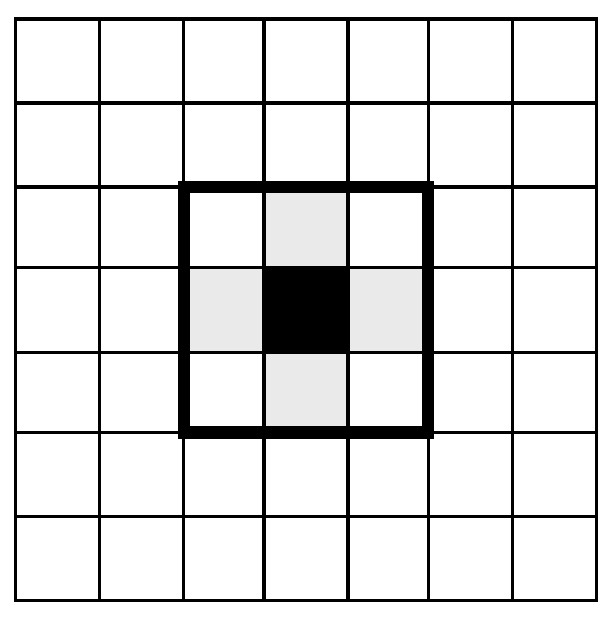
Example: Pixel neighbors in Moore’s algorithm

In the Moore neighborhood tracing algorithm, when the current pixel \(p\) is “black”, the Moore neighborhood of \(p\) is examined in a clockwise manner starting with the pixel from which p was entered and advancing pixel by pixel until a new “black” pixel in \(C\) is encountered as illustrated in the following figure:

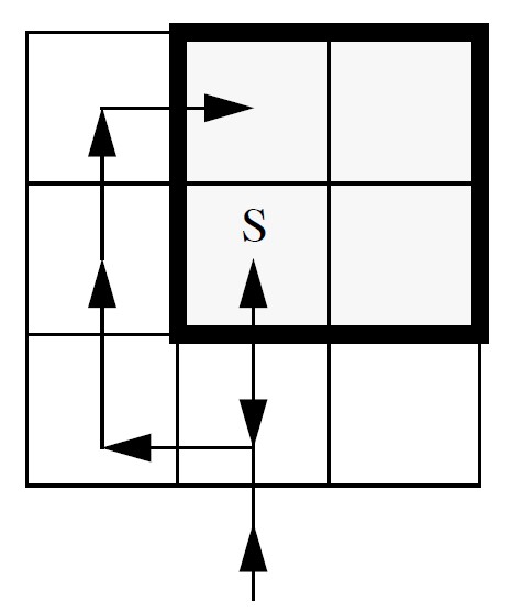
Example: Searching for the next “black” contour pixel in Moore-neighborhood contour tracing

The following figure shows an example of how the square tracing algorithm starting at the pixel marked \(S\) produces a sequence of boundary pixels in the case \(C\) is 8-connected:

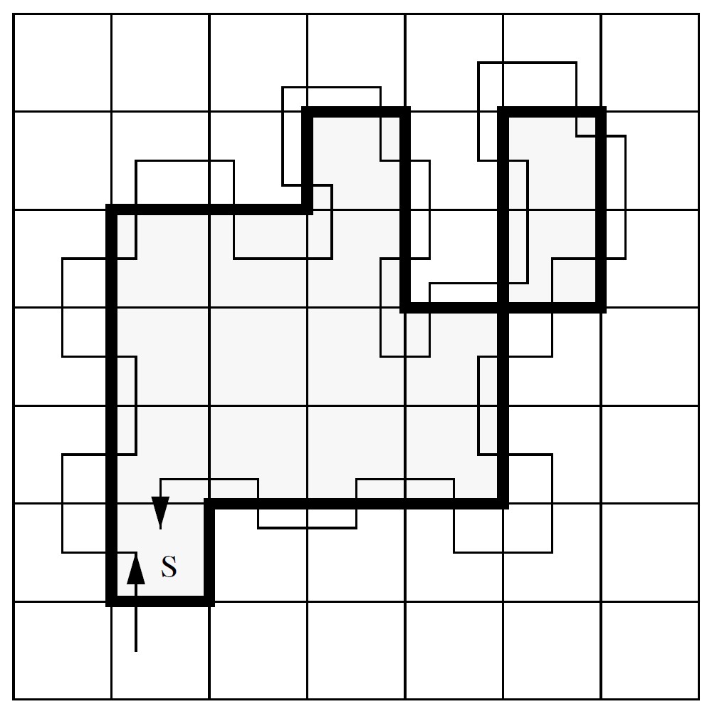
Example: Square tracing an 8-connected pattern

The algorithm is presented below:

Moore contour tracing algorithm:

Input: An image \(T\) containing a connected component \(C\) of “black” cells.

Output: A sequence \(B(b1, b2,..., bk)\) of boundary pixels.

begin

Step 1. Initialization: find a pixel in \(C\), initialize \(B\), define \(M(p)\) to be the Moore neighborhood of the current pixel \(p\).

Step 2. Set \(B\) to be empty.

Step 3. From bottom to top and left to right scan the cells of \(T\) until a pixel \(s\) of \(C\) is found (until the current pixel \(p=s\) is a “black” pixel of \(C\)), insert \(s\) in \(B\). Let \(b\) denote the current boundary point, i.e., \(b=s\).

Step 4. Backtrack (move the current pixel to the pixel from which \(s\) was entered) and advance the current pixel \(p\) being examined to the next clockwise pixel in \(M(b)\).

while (\(p \neq s\))

if (\(p\) is “black”)

insert \(p\) in \(B\);

set \(b=p\);

backtrack (move the current pixel to the pixel from which \(p=b\) was entered);

else

advance the current pixel \(p\) to the next clockwise pixel in \(M(b)\);

end-while

end

Note

1. Nyxus uses the region of interest mask, not intensity, image for contour tracing.

2. If a region of interest contains multiple contours, the outer contour is recognized with the contour tracing algorithm and used in calculation of contour-dependent features DIAMETER_MIN_ENCLOSING_CIRCLE, DIAMETER_INSCRIBING_CIRCLE, DIAMETER_CIRCUMSCRIBING_CIRCLE, POLYGONALITY_AVE, HEXAGONALITY_AVE, HEXAGONALITY_STDDEV, WEIGHTED_SPAT_MOMENT_pq, WEIGHTED_CENTRAL_MOMENT_pq, WEIGHTED_HU_M1-7, PERCENT_TOUCHING, FRAC_AT_D, MEAN_FRAC, and RADIAL_CV.

Features related to ROI’s contour

Let \(C\) be the set of contour pixels of ROI \(A\).

PERIMETER \(\gets P = card(C)\)

CIRCULARITY = \(\sqrt { \frac {4 \pi S}{P^2}}\) where \(S\) and \(P\) are ROI area and perimeter (features AREA_PIXELS_COUNT and PERIMETER)

EQUIVALENT_DIAMETER = \(\frac {P}{\pi}\)

EDGE_MEAN_INTENSITY \(\gets \mu_C =\frac{1}{card(C)}\sum_i C_i\)

EDGE_MAX_INTENSITY = \(\max \: \textrm C\)

EDGE_MIN_INTENSITY = \(\min \: \textrm C\)

EDGE_STDDEV_INTENSITY = \(\left[\frac{1}{card(C)}\sum_i (C_i-\mu_C)^2\right]^{\frac {1}{2}}\)

EDGE_INTEGRATEDINTENSITY = \(\sum _i {C_i}\)

Features related to ROI’s convex hull

CONVEX_HULL_AREA = \(S_H= {\frac {1}{2}}{\Biggl \vert }\sum _{i=0}^{n_H-1}(x_{i}y_{i+1}-x_{i+1}y_{i}){\Biggr \vert }\) where \(n_H\) is the number of convex hull vertices, \({(x_i,y_i)}, i=0, 1, ..., n_H-1\) are Cartesian coordinates of the vertives.

SOLIDITY = \(\frac {S}{S_H}\) where \(S\) is ROI area (feature AREA_PIXELS_COUNT)

Features related to interpreting ROI pixels as a sampled ellipse

MAJOR_AXIS_LENGTH \(= a = 4 \sqrt {\lambda_1}\) where \(\lambda_1\) is the first largest principal component

MINOR_AXIS_LENGTH \(= b = 4 \sqrt {\lambda_2}\) where \(\lambda_2\) is the second largest principal component

ECCENTRICITY \(= \sqrt {1 - \frac {b^2} {a^2}}\)

ELONGATION \(= \sqrt{\frac{\lambda_2}{\lambda_1}}\)

ORIENTATION \(\theta = 0\) if \(b=0\) and \(a \ge c \ \frac{\pi}{2}\) when \(b=0\) and \(a < c \ \arctan \frac{\lambda_1-a}{b}\) if \(b \ne 0\)

where

\[\begin{split}cov = \left(\begin{array}{cc} a & b \\ b & c \end{array}\right)\end{split}\]

is the covariance matrix of ROI pixel coordinates and

\[\begin{split}\lambda_1 &= \frac{a+c}{2}+\sqrt{(\frac{a-c}{2})^2 + b^2} \\ \lambda_2 &= \frac{a+c}{2}-\sqrt{(\frac{a-c}{2})^2 + b^2}\end{split}\]

ROUNDNESS = \(\frac {4 S}{\pi a b}\)

Neighbor features

NUM_NEIGHBORS \(\gets n_N=\) the number of neighbor ROIs

PERCENT_TOUCHING - the ratio of ROIs situated at Euclidean distance 0 to \(n_N\)

CLOSEST_NEIGHBOR1_DIST - distance to ROI’s closest neighbor

CLOSEST_NEIGHBOR1_ANG - angle between the ROI centroid and its closest neighbor’s centroid

CLOSEST_NEIGHBOR2_DIST - distance to ROI’s 2nd closest neighbor

CLOSEST_NEIGHBOR2_ANG - angle between the ROI centroid and its 2nd closest neighbor’s centroid

ANG_BW_NEIGHBORS_MEAN - standard deviation of the angle between ROI’s neighbors.

ANG_BW_NEIGHBORS_STDDEV - standard deviation of the angle between ROI’s neighbors.

ANG_BW_NEIGHBORS_MODE - the histogram bin value of angle between ROI’s neighbors having the highest count.

Polygonal representation features

POLYGONALITY_AVE = \(5 (r_S + r_A)\) where \(r_S = 1 - \left|1-\frac{\frac{P}{n_N}}{\sqrt{\frac{4S\tan \frac{\pi}{n_N}}{n_N}}} \right|\) - polygonal size \(r_A = 1 - \left| 1 - \frac{S\tan \frac{\pi}{n_N}}{\frac{1}{4} \: n_N \: P^2}\right|\) - polygonal area ratio, \(n_N\) - number of ROI’s neighbors, \(P\) and \(S\) - ROI’s perimeter and area.

HEXAGONALITY_AVE = \(\sqrt {\frac {r_{\sigma A}^2 + r_{\sigma P}^2}{2} }\)

HEXAGONALITY_STDDEV = \(5 (r_{HS} + r_{HP})\)

References: Nishi O, Hanasaki K. Automated determination of polygonality of corneal endothelial cells. Cornea. 1989;8(1):54-7. PMID: 2924585.

Other features

DIAMETER_MIN_ENCLOSING_CIRCLE minimum diameter of a circle which completely covers the ROI

DIAMETER_CIRCUMSCRIBING_CIRCLE the smallest circle centered at the ROI centroid that totally encloses the profile,

DIAMETER_INSCRIBING_CIRCLE maximum diameter of a circle centered at the ROI centroid which fits inside the ROI

Let \(l_G\) - geodetic length, \(t_G\) - thickness. Assuming

\[\begin{split}S &= l_G t_G \\ P &= 2(l_G+t_G)\end{split}\]

we can express the following features as:

GEODETIC_LENGTH \(\gets l_G = \frac{P}{4} + \sqrt{\max \left(\frac{P^2}{16}-S, 0\right)}\) THICKNESS \(\gets t_G = \frac{P}{2} - l_G\)

Let \(O=o_X,o_Y\) be the ROI centroid and \(OC_i\) - segment connecting centroid to an edge pixel \(i\). Then

ROI_RADIUS_MEAN \(\gets \mu_r =\frac{1}{card(C)}\sum_i ||OC_i||\)

ROI_RADIUS_MAX = \(\max OC_i\)

ROI_RADIUS_MEDIAN - median radius \(OC_i\)

Caliper features

Feret diameter

MIN_FERET_DIAMETER - minimum \(X_{Fe}\)

MAX_FERET_DIAMETER - maximum \(X_{Fe}\)

MIN_FERET_ANGLE - rotation angle delivering \(\min X_{Fe}\)

MAX_FERET_ANGLE - rotation angle delivering \(\max X_{Fe}\)

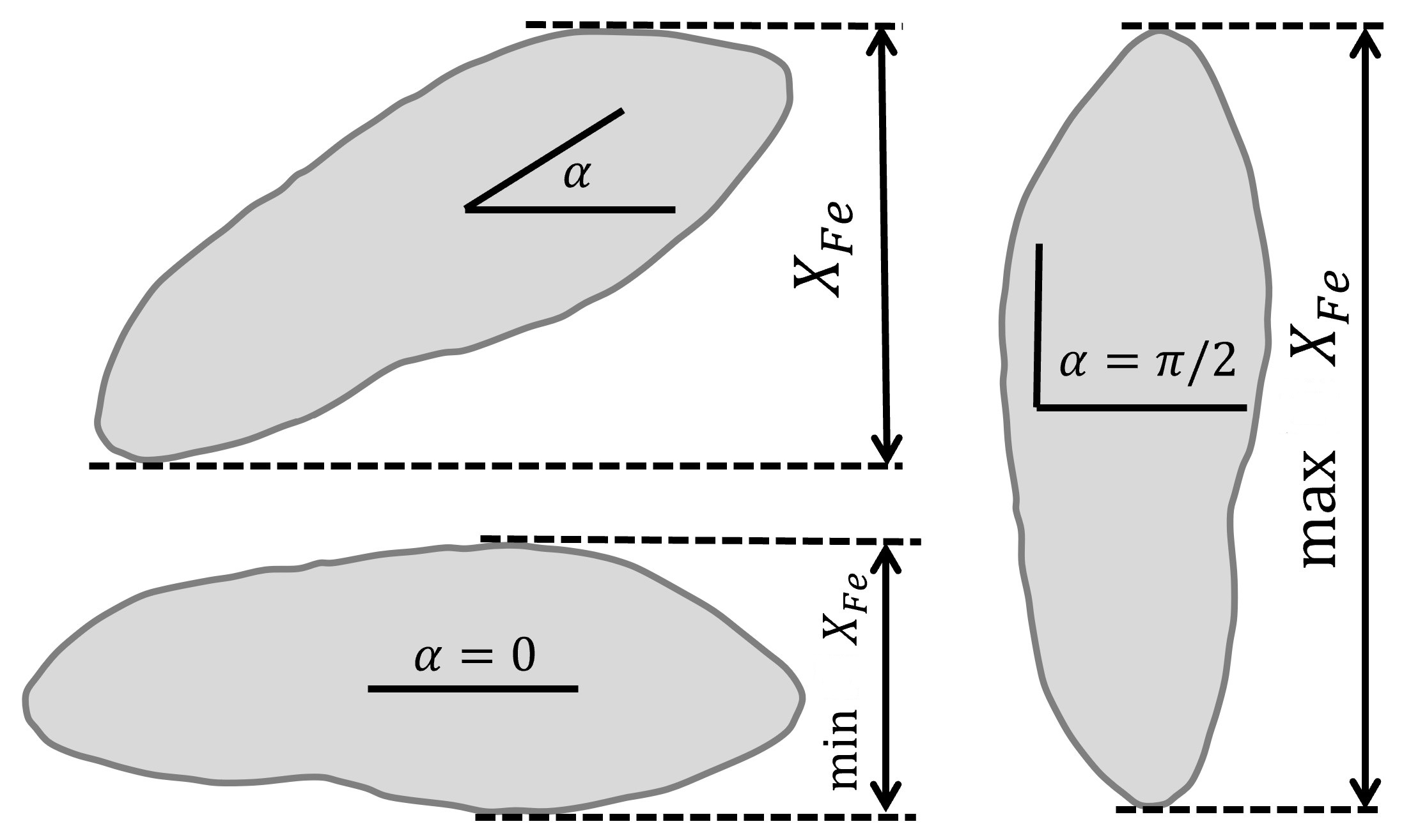
Statistics of Feret diameter at 0-90 degree rotation angles:

STAT_FERET_DIAM_MIN \(=\min X_{Fe}\)

STAT_FERET_DIAM_MAX \(=\max X_{Fe}\)

STAT_FERET_DIAM_MEAN \(=\operatorname {E} ( X_{Fe} )\)

STAT_FERET_DIAM_MEDIAN

STAT_FERET_DIAM_STDDEV

STAT_FERET_DIAM_MODE

Martin diameter

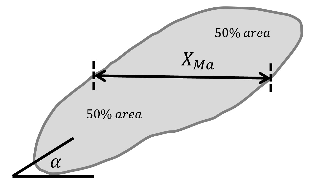
Statistics of Martin diameter at 0-90 degree rotation angles:

STAT_MARTIN_DIAM_MIN

STAT_MARTIN_DIAM_MAX

STAT_MARTIN_DIAM_MEAN

STAT_MARTIN_DIAM_MEDIAN

STAT_MARTIN_DIAM_STDDEV

STAT_MARTIN_DIAM_MODE

Nassenstein diameter

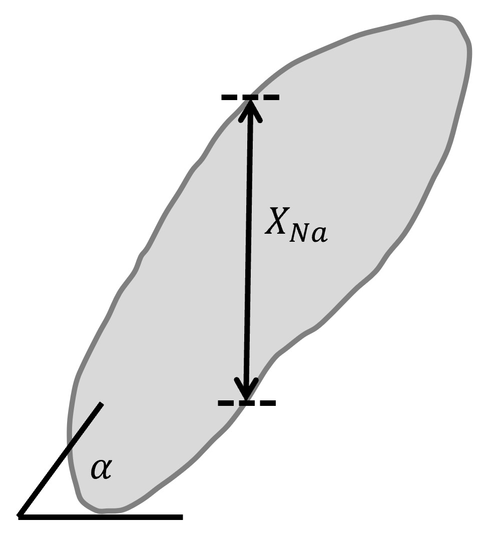
Statistics of Nassenstein diameter at 0-90 degree rotation angles:

|STAT_NASSENSTEIN_DIAM_MIN | STAT_NASSENSTEIN_DIAM_MAX | STAT_NASSENSTEIN_DIAM_MEAN | STAT_NASSENSTEIN_DIAM_MEDIAN | STAT_NASSENSTEIN_DIAM_STDDEV | STAT_NASSENSTEIN_DIAM_MODE

All-chords features

ALLCHORDS_MAX

ALLCHORDS_MAX_ANG

ALLCHORDS_MIN

ALLCHORDS_MIN_ANG

ALLCHORDS_MEDIAN

ALLCHORDS_MEAN

ALLCHORDS_MODE

ALLCHORDS_STDDEV

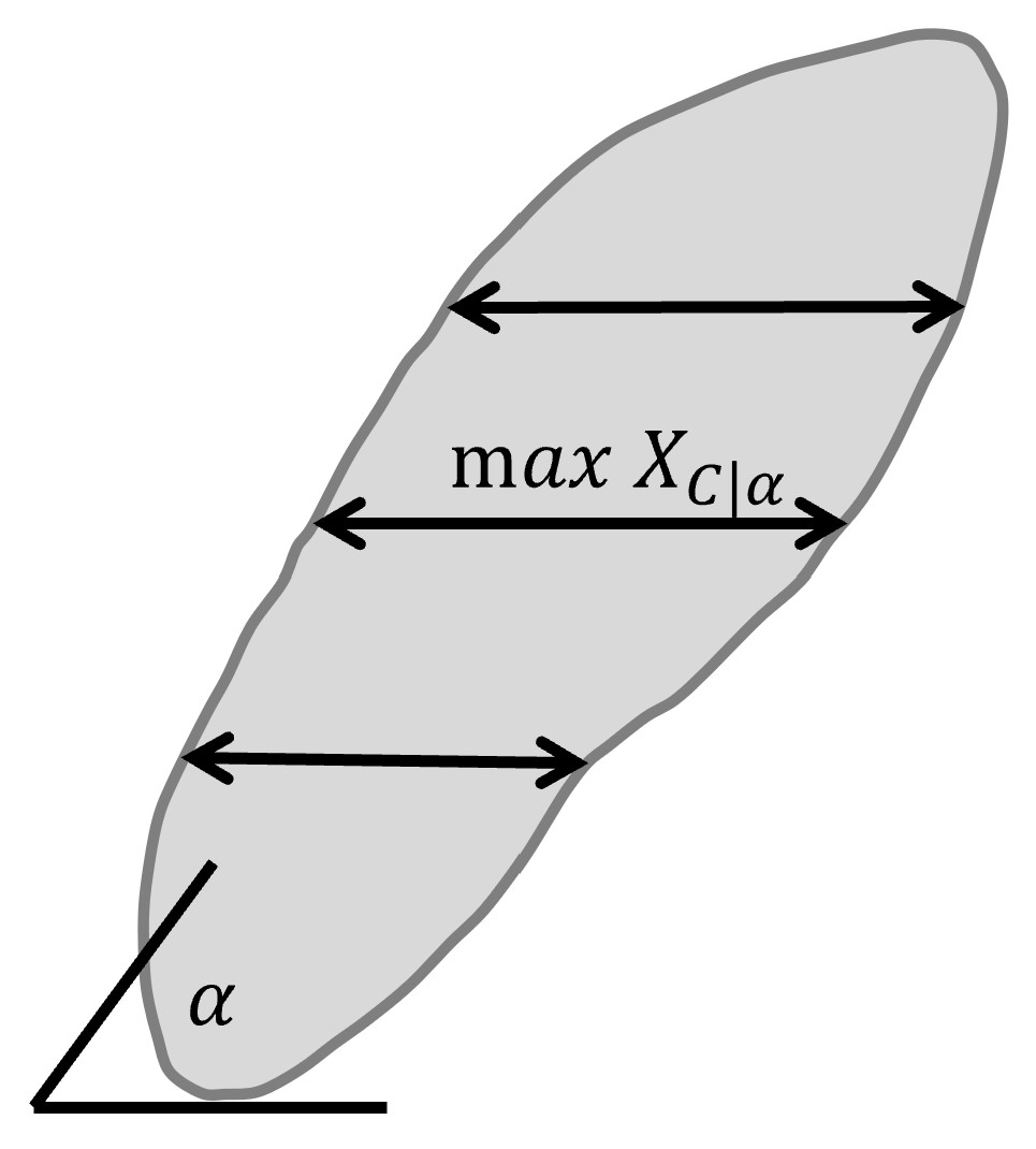
Max-chord features

MAXCHORDS_MAX

MAXCHORDS_MAX_ANG

MAXCHORDS_MIN

MAXCHORDS_MIN_ANG

MAXCHORDS_MEDIAN

MAXCHORDS_MEAN

MAXCHORDS_MODE

MAXCHORDS_STDDEV

References

1. Rosenfeld, A., “Digital topology,” American Mathematical Monthly, vol. 86, 1979, pp. 621-630.