Command line

Assuming you built the Nyxus executable from source code, the following parameters are available for the command line usage. Regular command line users should adhere parameter value to the “Type” column. WIPP developers should adhere to columns “WIPP I/O role” and “WIPP type”.

Parameter	Description	Type	WIPP I/O role	WIPP type
–outputType	Output type for feature values. Acceptable value: speratecsv, singlecsv, arrow, parquet. Default value: ‘–outputType=separatecsv’	string constant	input	enum
–features	String constant or comma-seperated list of constants requesting a group of features or particular feature. Default value: ‘–features=*ALL*’	string	input	array
–filePattern	Regular expression to match image files in directories specified by parameters ‘–intDir’ and ‘–segDir’. To match all the files, use ‘–filePattern=.*’	string	input	string
–intDir	Directory of intensity image collection	path	input	collection
–outDir	Output directory	path	output	csvCollection
–segDir	Directory of labeled image collection	path	input	collection
–coarseGrayDepth	(Optional) Custom number of grayscale level bins used in texture features. Default: ‘–coarseGrayDepth=256’	integer	input	integer
–gaborfreqs	(Optional) Feature GABOR: custom denominators of \(\pi\) as frequencies of Gabor filter’s harmonic factor. Default: ‘–gaborfreqs=1,2,4,8,16,32,64’	list of integer constants	input	collection
–gaborf0	(Optional) Feature GABOR: frequency of the baseline lowpass filter as denominator of \(\pi\). Default: ‘–gaborf0=0.1’	real	input	number
–gaborgamma	(Optional) Feature GABOR: aspect ratio of Gabor filter’s Gaussian factor. Default: ‘–gaborgamma=0.1’	real	input	number
–gaborkersize	(Optional) Feature GABOR: dimension of the 2D Gabor filter kernel. Default: ‘–gaborkersize=16’	integer	input	integer
–gaborsig2lam	(Optional) Feature GABOR: spatial frequency bandwidth of Gabor filter. Default: ‘–gaborsig2lam=0.8’	real	input	number
–gabortheta	(Optional) Feature GABOR: orientation of the Gaussian in degrees 0-180. Default: ‘–gabortheta=45’	real	input	number
–gaborthold	(Optional) Feature GABOR: lower threshold of the filtered image to baseline ratio. Default: ‘–gaborthold=0.025’	real	input	number
–glcmAngles	(Optional) Feature GLCM: enabled direction angles. Superset of values: 0, 45, 90, and 135. Default: ‘–glcmAngles=0,45,90,135’	list of integer constants	input	collection
–intSegMapDir	(Optional) Data collection of the ad-hoc intensity-to-mask file mapping. Must be used in combination with parameter ‘–intSegMapFile’	path	input	collection
–intSegMapFile	(Optional) Name of the text file containing an ad-hoc intensity-to-mask file mapping. The files are assumed to reside in corresponding intensity and label collections. Must be used in combination with parameter ‘–intSegMapDir’	string	input	string
–pixelDistance	(Optional) Number of pixels to treat ROIs within specified distance as neighbors. Default value: ‘–pixelDistance=5’	integer	input	integer
–pixelsPerCentimeter	(Optional) Number of pixels in centimeter used by unit length-related features. Default value: 0	real	input	number
–ramLimit	(Optional) Amount of memory not to exceed by Nyxus, in megabytes. Default value: 50% of available memory. Example: ‘–ramLimit=2000’ to use 2,000 megabytes	integer	input	integer
–reduceThreads	(Optional) Number of CPU threads used on the feature calculation step. Default: ‘–reduceThreads=1’	integer	input	integer
–skiproi	(Optional) Skip ROIs having specified labels. Example: ‘–skiproi=image1.tif:2,3,4;image2.tif:45,56’	string	input	string
–tempDir	(Optional) Directory used by temporary out-of-RAM objects. Default value: system temporary directory	path	input	path
–arrowOutputType	(Optional) Type of Arrow file to write the feature results to. Current options are ‘arrow’ for Arrow IPC or ‘parquet’ for Parquet	string	output	enum

Examples

This chapter presents some particular usage cases of Nyxus

1. Requesting specific features

Suppose we need to extract only Zernike features and first 3 Hu’s moments:

./nyxus --features=ZERNIKE2D,HU_M1,HU_M2,HU_M3 --intDir=/home/ec2-user/data-ratbrain/int --segDir=/home/ec2-user/data-ratbrain/seg --outDir=/home/ec2-user/work/OUTPUT-ratbrain --filePattern=.* --outputType=singlecsv

2. Requesting specific feature groups

Suppose we need to extract only intensity features basic morphology features:

./nyxus --features=*all_intensity*,*basic_morphology* --intDir=/home/ec2-user/data-ratbrain/int --segDir=/home/ec2-user/data-ratbrain/seg --outDir=/home/ec2-user/work/OUTPUT-ratbrain --filePattern=.* --outputType=singlecsv

3. Mixing specific feature groups and individual features

Suppose we need to extract intensity features, basic morphology features, and Zernike features:

./nyxus --features=*all_intensity*,*basic_morphology*,zernike2d --intDir=/home/ec2-user/data-ratbrain/int --segDir=/home/ec2-user/data-ratbrain/seg --outDir=/home/ec2-user/work/OUTPUT-ratbrain --filePattern=.* --outputType=singlecsv

4. Specifying a feature list from with a file instead of command line

Sometimes a list of requested features can be long making Nyxus command line huge. An alternative to dealing with a long command line is specifying all the desired features in a comma, space, and newline delimited text file. Suppose a feature set is in file feature_list.txt:

mean,min,kurtosis
skewness

Then the command line will be:

./nyxus --features=feature_list.txt --intDir=/home/ec2-user/data-ratbrain/int --segDir=/home/ec2-user/data-ratbrain/seg --outDir=/home/ec2-user/work/OUTPUT-ratbrain --filePattern=.* --outputType=singlecsv

5. Whole-image feature extraction

The regular operation mode of Nyxus is processing pairs of intensity and mask images treating non-zero pixel values of the mask image as segment label. The other operation mode is the so called “single-ROI mode” - treating the intensity image as segment. To activate it, just reference the intensity image collection as mask in the command line:

./nyxus --features=*basic_morphology* --intDir=/home/ec2-user/data-ratbrain/int --segDir=/home/ec2-user/data-ratbrain/int --outDir=/home/ec2-user/work/OUTPUT-ratbrain --filePattern=.* --outputType=singlecsv

6. Regular and ad-hoc mapping between intensity and mask image files

Intensity and mask image collections are specified in the command line (via parameters –intDir and –segDir) and the default mapping between an intensity and mask image, after applying a file name pattern (via parameter –filePattern), is the 1:1 mapping:

intensity_image_1       segment_image_1
intensity_image_2       segment_image_2
intensity_image_3       segment_image_3
intensity_image_4       segment_image_4

Here, each intensity and mask image is assumed to reside in the corresponding image collection directory specified with command line arguments –intDir=/home/ec2-user/data-ratbrain/int –segDir=/home/ec2-user/data-ratbrain/seg. More precisely:

/home/ec2-user/data-ratbrain/int/image_1.ome.tif    /home/ec2-user/data-ratbrain/seg/image_1.ome.tif
/home/ec2-user/data-ratbrain/int/image_2.ome.tif    /home/ec2-user/data-ratbrain/seg/image_2.ome.tif
/home/ec2-user/data-ratbrain/int/image_3.ome.tif    /home/ec2-user/data-ratbrain/seg/image_3.ome.tif
/home/ec2-user/data-ratbrain/int/image_4.ome.tif    /home/ec2-user/data-ratbrain/seg/image_4.ome.tif

In case the dataset is based on a 1:N mapping, for example

intensity_image_1       segment_image_A
intensity_image_2       segment_image_A
intensity_image_3       segment_image_A
intensity_image_4       segment_image_B

the user needs to pass such an ad-hoc mapping to Nyxus via referenceing a mapping definition text file in the command line (parameter –intSegMapFile).

Note: the order of mapping definition file columns is critical, and the 1-st column is interpreted as the intensity image files column while the 2-nd column is interpreted as the mask image files.

Assuming contents of file mapping.txt is

image_1.ome.tif       image_A.ome.tif
image_2.ome.tif       image_A.ome.tif
image_3.ome.tif       image_A.ome.tif
image_4.ome.tif       image_B.ome.tif

and the file is passed to Nyxus via parameter –intSegMapFile, the mapping will resolve to mapping

/home/ec2-user/data-ratbrain/int/image_1.ome.tif    /home/ec2-user/data-ratbrain/seg/image_A.ome.tif
/home/ec2-user/data-ratbrain/int/image_2.ome.tif    /home/ec2-user/data-ratbrain/seg/image_A.ome.tif
/home/ec2-user/data-ratbrain/int/image_3.ome.tif    /home/ec2-user/data-ratbrain/seg/image_A.ome.tif
/home/ec2-user/data-ratbrain/int/image_4.ome.tif    /home/ec2-user/data-ratbrain/seg/image_B.ome.tif

7. Ad-hoc mapping between intensity and mask image files via Python interface

Alternatively, Nyxus can process explicitly defined pairs of intensity-mask images, for example image “i1” with mask “m1” and image “i2” with mask “m2”:

from nyxus import Nyxus
nyx = Nyxus(["*ALL*"])
features = nyx.featurize_files(
   [
      "/path/to/images/intensities/i1.ome.tif",
      "/path/to/images/intensities/i2.ome.tif"
   ],
   [
      "/path/to/images/labels/m1.ome.tif",
      "/path/to/images/labels/m2.ome.tif"
   ])

Nyxus can also process intensity-mask pairs that are stored as Numpy arrays using the featurize method. This method takes in either a single pair of 2D intensity-mask pairs or a pair of 3D arrays containing 2D intensity and mask images. There is also two optional parameters to supply names to the resulting dataframe, .

from nyxus import Nyxus
import numpy as np

nyx = Nyxus(["*ALL*"])

intens = [
   [[1, 4, 4, 1, 1],
   [1, 4, 6, 1, 1],
   [4, 1, 6, 4, 1],
   [4, 4, 6, 4, 1]],

   [[1, 4, 4, 1, 1],
   [1, 1, 6, 1, 1],
   [1, 1, 3, 1, 1],
   [4, 4, 6, 1, 1]]
]

seg = [
   [[1, 1, 1, 1, 1],
   [1, 1, 1, 1, 1],
   [1, 1, 1, 1, 1],
   [1, 1, 1, 1, 1]],

   [[1, 1, 1, 1, 1],
   [1, 1, 1, 1, 1],
   [0, 1, 1, 1, 1],
   [1, 1, 1, 1, 1]]
]


features = nyx.featurize(intens, seg)

The features variable is a Pandas dataframe similar to what is shown below.

     mask_image     intensity_image  label  MEAN       MEDIAN   ...  GABOR_6

0   Segmentation1   Intensity1         1    45366.9    46887    ...  0.873016
1   Segmentation1   Intensity1         2    27122.8    27124.5  ...  1.000000
2   Segmentation1   Intensity1         3    34777.4    33659    ...  0.942857
3   Segmentation1   Intensity1         4    35808.2    36924    ...  0.824074
...    ...             ...            ...     ...      ...      ...    ...
14  Segmentation2   Intensity2         6    54573.3    54573.3  ...  0.980769

Note that in this case, default names were provided for the mask_image and intensity_image columns. To supply names for these columns, the optional arguments intensity_names and label_names are used by passing lists of names in. The length of the lists must be the same as the length of the mask and intensity arrays. To name the images, use

intens_names = ['custom_intens_name1', 'custom_intens_name2']
seg_names = ['custom_seg_name1', 'custom_seg_name2']

features = nyx.featurize(intens, seg, intens_name, seg_name)

The features variable will now use the custom names, as shown below

    mask_image        intensity_image             label  MEAN       MEDIAN   ...  GABOR_6

0   custom_seg_name1   custom_intens_name1          1    45366.9    46887    ...  0.873016
1   custom_seg_name1   custom_intens_name1          2    27122.8    27124.5  ...  1.000000
2   custom_seg_name1   custom_intens_name1          3    34777.4    33659    ...  0.942857
3   custom_seg_name1   custom_intens_name1          4    35808.2    36924    ...  0.824074
...    ...             ...            ...     ...      ...      ...    ...
14  custom_seg_name2   Intensity2         6    54573.3    54573.3  ...  0.980769

All parameters to configure Nyxus are available to set within the constructor. These parameters can also be updated after the object is created using the set_params method. This method takes in keyword arguments where the key is a valid parameter in Nyxus and the value is the updated value for the parameter. For example, to update the coarse_gray_depth to 256 and the gabor_f0 parameter to 0.1, the following can be done:

from nyxus import Nyxus
nyx = Nyxus(["*ALL*"])
intensityDir = "/path/to/images/intensities/"
maskDir = "/path/to/images/labels/"
features = nyx.featurize_directory (intensityDir, maskDir)

nyx.set_params(coarse_gray_depth=256, gabor_f0=0.1)

A list of valid parameters is included in the documentation for this method.

To get the values of the parameters in Nyxus, the get_params method is used. If no arguments are passed to this function, then a dictionary mapping all of the variable names to the respective value is returned. For example,

from nyxus import Nyxus
nyx = Nyxus(["*ALL*"])
intensityDir = "/path/to/images/intensities/"
maskDir = "/path/to/images/labels/"
features = nyx.featurize_directory (intensityDir, maskDir)

print(nyx.get_params())

will print the dictionary

{'coarse_gray_depth': 256,
'features': ['*ALL*'],
'gabor_f0': 0.1,
'gabor_freqs': [1.0, 2.0, 4.0, 8.0, 16.0, 32.0, 64.0],
'gabor_gamma': 0.1,
'gabor_kersize': 16,
'gabor_sig2lam': 0.8,
'gabor_theta': 45.0,
'gabor_thold': 0.025,
'ibsi': 0,
'n_loader_threads': 1,
'n_feature_calc_threads': 4,
'neighbor_distance': 5,
'pixels_per_micron': 1.0}

There is also the option to pass arguments to this function to only receive a subset of parameter values. The arguments should be valid parameter names as string, separated by commas. For example,

from nyxus import Nyxus
nyx = Nyxus(["*ALL*"])
intensityDir = "/path/to/images/intensities/"
maskDir = "/path/to/images/labels/"
features = nyx.featurize_directory (intensityDir, maskDir)

print(nyx.get_params('coarse_gray_depth', 'features', 'gabor_f0'))

will print the dictionary

{'coarse_gray_depth': 256,
'features': ['*ALL*'],
'gabor_f0': 0.1}

8. Using Arrow for feature results

Nyxus provides the ability to get the results of the feature calculations in Arrow IPC and Parquet formats. To create an Arrow IPC or Parquet file, use output_type=”arrowipc” or output_type=”parquet” in Nyxus.featurize* calls. Optionally, an output_path argument can be passed to specify the location of the output file.

from nyxus import Nyxus
import numpy as np

intens = np.array([
   [[1, 4, 4, 1, 1],
   [1, 4, 6, 1, 1],
   [4, 1, 6, 4, 1],
   [4, 4, 6, 4, 1]],

   [[1, 4, 4, 1, 1],
   [1, 1, 6, 1, 1],
   [1, 1, 3, 1, 1],
   [4, 4, 6, 1, 1]],

   [[1, 4, 4, 1, 1],
   [1, 1, 1, 1, 1],
   [1, 1, 6, 1, 1],
   [1, 1, 6, 1, 1]],

   [[1, 4, 4, 1, 1],
   [1, 1, 1, 1, 1],
   [1, 1, 1, 1, 1],
   [1, 1, 6, 1, 1]],
])

seg = np.array([
   [[1, 1, 1, 1, 1],
   [1, 1, 1, 1, 1],
   [1, 1, 1, 1, 1],
   [1, 1, 1, 1, 1]],

   [[1, 1, 1, 1, 1],
   [1, 1, 1, 1, 1],
   [0, 1, 1, 1, 1],
   [1, 1, 1, 1, 1]],

   [[1, 1, 1, 0, 0],
   [1, 1, 1, 1, 1],
   [1, 1, 0, 1, 1],
   [1, 1, 1, 1, 1]],

   [[1, 1, 1, 0, 0],
   [1, 1, 1, 1, 1],
   [1, 1, 1, 1, 1],
   [1, 1, 1, 1, 1]]

])

nyx = Nyxus(["*ALL_INTENSITY*"])

arrow_file = nyx.featurize(intens, seg, output_type="arrowipc", output_path="some_path")

print(arrow_file)

The output is:

some_path/NyxusFeatures.arrow

9. Nested Features Examples

The Nested class is the Python API of Nyxus identifies child-parent relations of ROIs in images with a child and parent channel. For example, consider the following intensity and segmentation images of the parent channel,

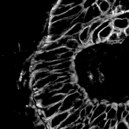
Fig 1. Parent channel intensity

Fig 2. Parent channel segmentation

With the child channel

Fig 3. Child channel intensity

Fig 4. Child channel segmentation

As shown by the figures, there are ROIs in the child segmentation that are completely contained in the the ROIs of the parent channel. The purpose of the Nested class is to identify the child ROIs of the parent channel. The Nested class also contains functionality to apply aggregate functions to the child features, as shown belong in the example.

To use the Nested class, first call the constructor with the optional argument aggregate. If aggregate is not passed, the find_relation behavior will change (described later). Any aggregate function supported by Pandas is available, such as min, max, count, and mean. Lambda functions can also be used, and named using a 2-tuple, where the first element is the name and the second is the lambda function. This allows functions that are not supported by Pandas to be used, such as Numpy’s np.nanmean.

To use the Nested class, first call Nyxus to get the features of all ROIs from the child channels. If the child channels are described by a channel number in the filename, a filepattern can be used to filter down to only the child channel. Consider a directory with the images

p0_y1_r1_c0.ome.tif
p0_y1_r1_c1.ome.tif
p0_y1_r2_c0.ome.tif
p0_y1_r2_1.ome.tif
p0_y1_r3_c0.ome.tif
p0_y1_r3_c1.ome.tif
...

where the child channel is designated by c0 and the parent channel is c1. We can filter down to only the child channel using the filepattern p{r}_y{c}_r{z}_c0.ome.tif or the equivalent regex p[0-9]_y[0-9]_r[0-9]_c0.ome.tif.

Next, we calculate the features for the child channel. For simplicity, we only use the Gabor features, but any or all features can be used.

from nyxus import Nyxus, Nested
import numpy as np

int_path = 'path/to/intensity'
seg_path = 'path/to/segmentation'

nyx = Nyxus(['GABOR'])

child_features = nyx.featurize(int_path, seg_path, file_pattern='p[0-9]_y[0-9]_r[0-9]_c0\.ome\.tif')

print(features.head())

The result of this code is

mask_image                    intensity_image  label   GABOR_0   GABOR_1   GABOR_2   GABOR_3   GABOR_4   GABOR_5   GABOR_6
0    p0_y1_r1_c0.ome.tif  p0_y1_r1_c0.ome.tif      1  0.224206  0.172619  0.166667  0.730159  0.773810  0.767857  0.753968
1    p0_y1_r1_c0.ome.tif  p0_y1_r1_c0.ome.tif      2  1.000000  0.610000  0.540000  0.980000  0.990000  0.990000  0.970000
2    p0_y1_r1_c0.ome.tif  p0_y1_r1_c0.ome.tif      3  0.429864  0.217195  0.122172  0.877828  0.941176  0.936652  0.909502
3    p0_y1_r1_c0.ome.tif  p0_y1_r1_c0.ome.tif      4  0.846154  0.948718  0.717949  1.000000  1.000000  1.000000  1.000000
4    p0_y1_r1_c0.ome.tif  p0_y1_r1_c0.ome.tif      5  0.277778  0.021368  0.029915  0.794872  0.841880  0.841880  0.824786

Next, the find_relation method is used to find the child-parent relations. This method takes in the segmentation path along with filepatterns to distinguish the child channel from the parent channel.

nest = Nested(['sum', 'mean', 'min', ('nanmean', lambda x: np.nanmean(x))])

df = nest.find_relations(seg_path, 'p{r}_y{c}_r{z}_c1.ome.tif', 'p{r}_y{c}_r{z}_c0.ome.tif')
print(df.head())

The result is

Image              Parent_Label  Child_Label
0  /path/to/image          72.0         65.0
1  /path/to/image          71.0         66.0
2  /path/to/image          70.0         64.0
3  /path/to/image          68.0         61.0
4  /path/to/image          67.0         65.0

The featurize method can then be used along with the child features to apply the aggregate functions. The featurize method takes in the features DataFrame generated by Nyxus, which contains the features calculations for each ROI, along with the DataFrame containing the parent-child relations from the find_relations method. The output of this method is a DataFrame containing

df = nest.featurize(df, features)
print(df.head())

The result is

GABOR_0                                  GABOR_1                                  GABOR_2            ...   GABOR_4              GABOR_5                                  GABOR_6
        sum      mean       min   nanmean        sum      mean       min   nanmean        sum      mean  ...       min   nanmean        sum      mean       min   nanmean        sum      mean       min   nanmean
label                                                                                                         ...
1      24.010227  0.666951  0.000000  0.666951  19.096262  0.530452  0.001645  0.530452  17.037345  0.473260  ...  0.773810  0.897924  32.060053  0.890557  0.767857  0.890557  31.643434  0.878984  0.753968  0.878984
2      13.374170  0.445806  0.087339  0.445806   7.279187  0.242640  0.075000  0.242640   6.390529  0.213018  ...  0.735000  0.885494  26.414860  0.880495  0.727500  0.880495  25.886468  0.862882  0.700000  0.862882
3       5.941783  0.198059  0.000000  0.198059   3.364149  0.112138  0.000000  0.112138   2.426409  0.080880  ...  0.858462  0.900500  26.836040  0.894535  0.858462  0.894535  26.172914  0.872430  0.829231  0.872430
4      13.428773  0.559532  0.000000  0.559532  12.021938  0.500914  0.008772  0.500914   9.938915  0.414121  ...  0.820175  0.945459  22.572913  0.940538  0.802632  0.940538  22.270382  0.927933  0.787281  0.927933
5       6.535722  0.181548  0.000000  0.181548   1.833463  0.050930  0.000000  0.050930   2.083023  0.057862  ...  0.697917  0.819318  29.094328  0.808176  0.693452  0.808176  28.427727  0.789659  0.675595  0.789659

The other way to utilize the Nested class is to not pass any aggregate features to the constructor. In this case, the featurize method with create a pivot table where the rows are the ROI labels and the columns are grouped by the features.

nest = Nested(['sum', 'mean', 'min', ('nanmean', lambda x: np.nanmean(x))])

df = nest.find_relations(seg_path, 'p{r}_y{c}_r{z}_c1.ome.tif', 'p{r}_y{c}_r{z}_c0.ome.tif')

df = nest.featurize(df, features)
print(df.head())

The result is

              GABOR_0                                                                   ... GABOR_6
Child_Label      1.0       2.0       3.0       4.0       5.0  6.0  7.0  8.0  9.0  10.0  ...    55.0 56.0 58.0 59.0 60.0 61.0 62.0 64.0 65.0 66.0
label                                                                                   ...
1            0.666951       NaN       NaN       NaN       NaN  NaN  NaN  NaN  NaN  NaN  ...     NaN  NaN  NaN  NaN  NaN  NaN  NaN  NaN  NaN  NaN
2                 NaN  0.445806       NaN       NaN       NaN  NaN  NaN  NaN  NaN  NaN  ...     NaN  NaN  NaN  NaN  NaN  NaN  NaN  NaN  NaN  NaN
3                 NaN       NaN  0.198059       NaN       NaN  NaN  NaN  NaN  NaN  NaN  ...     NaN  NaN  NaN  NaN  NaN  NaN  NaN  NaN  NaN  NaN
4                 NaN       NaN       NaN  0.559532       NaN  NaN  NaN  NaN  NaN  NaN  ...     NaN  NaN  NaN  NaN  NaN  NaN  NaN  NaN  NaN  NaN
5                 NaN       NaN       NaN       NaN  0.181548  NaN  NaN  NaN  NaN  NaN  ...     NaN  NaN  NaN  NaN  NaN  NaN  NaN  NaN  NaN  NaN