Examples
This chapter presents some particular usage cases of Nyxus
1. Requesting specific features
Suppose we need to extract only Zernike features and first 3 Hu’s moments:
./nyxus --features=ZERNIKE2D,HU_M1,HU_M2,HU_M3 --intDir=/home/ec2-user/data-ratbrain/int --segDir=/home/ec2-user/data-ratbrain/seg --outDir=/home/ec2-user/work/OUTPUT-ratbrain --filePattern=.* --csvFile=singlecsv
2. Requesting specific feature groups
Suppose we need to extract only intensity features basic morphology features:
./nyxus --features=*all_intensity*,*basic_morphology* --intDir=/home/ec2-user/data-ratbrain/int --segDir=/home/ec2-user/data-ratbrain/seg --outDir=/home/ec2-user/work/OUTPUT-ratbrain --filePattern=.* --csvFile=singlecsv
3. Mixing specific feature groups and individual features
Suppose we need to extract intensity features, basic morphology features, and Zernike features:
./nyxus --features=*all_intensity*,*basic_morphology*,zernike2d --intDir=/home/ec2-user/data-ratbrain/int --segDir=/home/ec2-user/data-ratbrain/seg --outDir=/home/ec2-user/work/OUTPUT-ratbrain --filePattern=.* --csvFile=singlecsv
4. Specifying a feature list from with a file instead of command line
Sometimes a list of requested features can be long making Nyxus command line huge. An alternative to dealing with a long command line is specifying all the desired features in a comma, space, and newline delimited text file. Suppose a feature set is in file feature_list.txt:
mean,min,kurtosis
skewness
Then the command line will be:
./nyxus --features=feature_list.txt --intDir=/home/ec2-user/data-ratbrain/int --segDir=/home/ec2-user/data-ratbrain/seg --outDir=/home/ec2-user/work/OUTPUT-ratbrain --filePattern=.* --csvFile=singlecsv
5. Whole-image feature extraction
The regular operation mode of Nyxus is processing pairs of intensity and mask images treating non-zero pixel values of the mask image as segment label. The other operation mode is the so called “single-ROI mode” - treating the intensity image as segment. To activate it, just reference the intensity image collection as mask in the command line:
./nyxus --features=*basic_morphology* --intDir=/home/ec2-user/data-ratbrain/int --segDir=/home/ec2-user/data-ratbrain/int --outDir=/home/ec2-user/work/OUTPUT-ratbrain --filePattern=.* --csvFile=singlecsv
6. Regular and ad-hoc mapping between intensity and mask image files
Intensity and mask image collections are specified in the command line (via parameters –intDir and –segDir) and the default mapping between an intensity and mask image, after applying a file name pattern (via parameter –filePattern), is the 1:1 mapping:
intensity_image_1       segment_image_1
intensity_image_2       segment_image_2
intensity_image_3       segment_image_3
intensity_image_4       segment_image_4
Here, each intensity and mask image is assumed to reside in the corresponding image collection directory specified with command line arguments –intDir=/home/ec2-user/data-ratbrain/int –segDir=/home/ec2-user/data-ratbrain/seg. More precisely:
/home/ec2-user/data-ratbrain/int/image_1.ome.tif    /home/ec2-user/data-ratbrain/seg/image_1.ome.tif
/home/ec2-user/data-ratbrain/int/image_2.ome.tif    /home/ec2-user/data-ratbrain/seg/image_2.ome.tif
/home/ec2-user/data-ratbrain/int/image_3.ome.tif    /home/ec2-user/data-ratbrain/seg/image_3.ome.tif
/home/ec2-user/data-ratbrain/int/image_4.ome.tif    /home/ec2-user/data-ratbrain/seg/image_4.ome.tif
In case the dataset is based on a 1:N mapping, for example
intensity_image_1       segment_image_A
intensity_image_2       segment_image_A
intensity_image_3       segment_image_A
intensity_image_4       segment_image_B
the user needs to pass such an ad-hoc mapping to Nyxus via referenceing a mapping definition text file in the command line (parameter –intSegMapFile).
Note: the order of mapping definition file columns is critical, and the 1-st column is interpreted as the intensity image files column while the 2-nd column is interpreted as the mask image files.
Assuming contents of file mapping.txt is
image_1.ome.tif       image_A.ome.tif
image_2.ome.tif       image_A.ome.tif
image_3.ome.tif       image_A.ome.tif
image_4.ome.tif       image_B.ome.tif
and the file is passed to Nyxus via parameter –intSegMapFile, the mapping will resolve to mapping
/home/ec2-user/data-ratbrain/int/image_1.ome.tif    /home/ec2-user/data-ratbrain/seg/image_A.ome.tif
/home/ec2-user/data-ratbrain/int/image_2.ome.tif    /home/ec2-user/data-ratbrain/seg/image_A.ome.tif
/home/ec2-user/data-ratbrain/int/image_3.ome.tif    /home/ec2-user/data-ratbrain/seg/image_A.ome.tif
/home/ec2-user/data-ratbrain/int/image_4.ome.tif    /home/ec2-user/data-ratbrain/seg/image_B.ome.tif
7. Ad-hoc mapping between intensity and mask image files via Python interface
Alternatively, Nyxus can process explicitly defined pairs of intensity-mask images, for example image “i1” with mask “m1” and image “i2” with mask “m2”:
```python from nyxus import Nyxus nyx = Nyxus([”ALL”]) features = nyx.featurize(
- [
“/path/to/images/intensities/i1.ome.tif”, “/path/to/images/intensities/i2.ome.tif”
], [
“/path/to/images/labels/m1.ome.tif”, “/path/to/images/labels/m2.ome.tif”
])
8. Nested Features Examples
The Nested class is the Python API of Nyxus identifies child-parent relations of ROIs in images with a child and parent channel. For example, consider the following intensity and segmentation images of the parent channel,
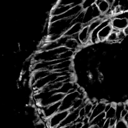
Fig 1. Parent channel intensity |

Fig 2. Parent channel segmentation |
With the child channel
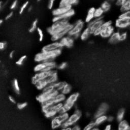
Fig 3. Child channel intensity |

Fig 4. Child channel segmentation |
As shown by the figures, there are ROIs in the child segmentation that are completely contained in the the ROIs of the parent channel. The purpose of the Nested class is to identify the child ROIs of the parent channel. The Nested class also contains functionality to apply aggregate functions to the child features, as shown belong in the example.
To use the Nested class, first call the constructor with the optional argument aggregate. If aggregate is not passed, the find_relation behavior will change (described later). Any aggregate function supported by Pandas is available, such as min, max, count, and mean. Lambda functions can also be used, and named using a 2-tuple, where the first element is the name and the second is the lambda function. This allows functions that are not supported by Pandas to be used, such as Numpy’s np.nanmean.
To use the Nested class, first call Nyxus to get the features of all ROIs from the child channels. If the child channels are described by a channel number in the filename, a filepattern can be used to filter down to only the child channel. Consider a directory with the images
p0_y1_r1_c0.ome.tif
p0_y1_r1_c1.ome.tif
p0_y1_r2_c0.ome.tif
p0_y1_r2_1.ome.tif
p0_y1_r3_c0.ome.tif
p0_y1_r3_c1.ome.tif
...
where the child channel is designated by c0 and the parent channel is c1. We can filter down to only the child channel using the filepattern p{r}_y{c}_r{z}_c0.ome.tif or the equivalent regex p[0-9]_y[0-9]_r[0-9]_c0.ome.tif.
Next, we calculate the features for the child channel. For simplicity, we only use the Gabor features, but any or all features can be used.
from nyxus import Nyxus, Nested
import numpy as np

int_path = 'path/to/intensity'
seg_path = 'path/to/segmentation'

nyx = Nyxus(['GABOR'])

child_features = nyx.featurize(int_path, seg_path, file_pattern='p[0-9]_y[0-9]_r[0-9]_c0\.ome\.tif')

print(features.head())
The result of this code is
mask_image                    intensity_image  label   GABOR_0   GABOR_1   GABOR_2   GABOR_3   GABOR_4   GABOR_5   GABOR_6
0    p0_y1_r1_c0.ome.tif  p0_y1_r1_c0.ome.tif      1  0.224206  0.172619  0.166667  0.730159  0.773810  0.767857  0.753968
1    p0_y1_r1_c0.ome.tif  p0_y1_r1_c0.ome.tif      2  1.000000  0.610000  0.540000  0.980000  0.990000  0.990000  0.970000
2    p0_y1_r1_c0.ome.tif  p0_y1_r1_c0.ome.tif      3  0.429864  0.217195  0.122172  0.877828  0.941176  0.936652  0.909502
3    p0_y1_r1_c0.ome.tif  p0_y1_r1_c0.ome.tif      4  0.846154  0.948718  0.717949  1.000000  1.000000  1.000000  1.000000
4    p0_y1_r1_c0.ome.tif  p0_y1_r1_c0.ome.tif      5  0.277778  0.021368  0.029915  0.794872  0.841880  0.841880  0.824786
Next, the find_relation method is used to find the child-parent relations. This method takes in the segmentation path along with filepatterns to distinguish the child channel from the parent channel.
nest = Nested(['sum', 'mean', 'min', ('nanmean', lambda x: np.nanmean(x))])

df = nest.find_relations(seg_path, 'p{r}_y{c}_r{z}_c1.ome.tif', 'p{r}_y{c}_r{z}_c0.ome.tif')
print(df.head())
The result is
Image              Parent_Label  Child_Label
0  /path/to/image          72.0         65.0
1  /path/to/image          71.0         66.0
2  /path/to/image          70.0         64.0
3  /path/to/image          68.0         61.0
4  /path/to/image          67.0         65.0
The featurize method can then be used along with the child features to apply the aggregate functions. The featurize method takes in the features DataFrame generated by Nyxus, which contains the features calculations for each ROI, along with the DataFrame containing the parent-child relations from the find_relations method. The output of this method is a DataFrame containing
df = nest.featurize(df, features)
print(df.head())
The result is
GABOR_0                                  GABOR_1                                  GABOR_2            ...   GABOR_4              GABOR_5                                  GABOR_6
        sum      mean       min   nanmean        sum      mean       min   nanmean        sum      mean  ...       min   nanmean        sum      mean       min   nanmean        sum      mean       min   nanmean
label                                                                                                         ...
1      24.010227  0.666951  0.000000  0.666951  19.096262  0.530452  0.001645  0.530452  17.037345  0.473260  ...  0.773810  0.897924  32.060053  0.890557  0.767857  0.890557  31.643434  0.878984  0.753968  0.878984
2      13.374170  0.445806  0.087339  0.445806   7.279187  0.242640  0.075000  0.242640   6.390529  0.213018  ...  0.735000  0.885494  26.414860  0.880495  0.727500  0.880495  25.886468  0.862882  0.700000  0.862882
3       5.941783  0.198059  0.000000  0.198059   3.364149  0.112138  0.000000  0.112138   2.426409  0.080880  ...  0.858462  0.900500  26.836040  0.894535  0.858462  0.894535  26.172914  0.872430  0.829231  0.872430
4      13.428773  0.559532  0.000000  0.559532  12.021938  0.500914  0.008772  0.500914   9.938915  0.414121  ...  0.820175  0.945459  22.572913  0.940538  0.802632  0.940538  22.270382  0.927933  0.787281  0.927933
5       6.535722  0.181548  0.000000  0.181548   1.833463  0.050930  0.000000  0.050930   2.083023  0.057862  ...  0.697917  0.819318  29.094328  0.808176  0.693452  0.808176  28.427727  0.789659  0.675595  0.789659
The other way to utilize the Nested class is to not pass any aggregate features to the constructor. In this case, the featurize method with create a pivot table where the rows are the ROI labels and the columns are grouped by the features.
nest = Nested(['sum', 'mean', 'min', ('nanmean', lambda x: np.nanmean(x))])

df = nest.find_relations(seg_path, 'p{r}_y{c}_r{z}_c1.ome.tif', 'p{r}_y{c}_r{z}_c0.ome.tif')

df = nest.featurize(df, features)
print(df.head())
The result is
              GABOR_0                                                                   ... GABOR_6
Child_Label      1.0       2.0       3.0       4.0       5.0  6.0  7.0  8.0  9.0  10.0  ...    55.0 56.0 58.0 59.0 60.0 61.0 62.0 64.0 65.0 66.0
label                                                                                   ...
1            0.666951       NaN       NaN       NaN       NaN  NaN  NaN  NaN  NaN  NaN  ...     NaN  NaN  NaN  NaN  NaN  NaN  NaN  NaN  NaN  NaN
2                 NaN  0.445806       NaN       NaN       NaN  NaN  NaN  NaN  NaN  NaN  ...     NaN  NaN  NaN  NaN  NaN  NaN  NaN  NaN  NaN  NaN
3                 NaN       NaN  0.198059       NaN       NaN  NaN  NaN  NaN  NaN  NaN  ...     NaN  NaN  NaN  NaN  NaN  NaN  NaN  NaN  NaN  NaN
4                 NaN       NaN       NaN  0.559532       NaN  NaN  NaN  NaN  NaN  NaN  ...     NaN  NaN  NaN  NaN  NaN  NaN  NaN  NaN  NaN  NaN
5                 NaN       NaN       NaN       NaN  0.181548  NaN  NaN  NaN  NaN  NaN  ...     NaN  NaN  NaN  NaN  NaN  NaN  NaN  NaN  NaN  NaN